Paper Github Repo Quick Start

Visuomotor policies were often slow

Speed remains a bottleneck in visuomotor policies. A key reason is action chunking: policies predict fixed-rate waypoints, treating every moment the same. Manipulation is not uniform: robots should move fast in free space and slow down near contact making. Simply speeding up these waypoints can make motion jerky, and hard to track.

To address these issues, we propose B-spline Policy. Instead of predicting fixed-rate waypoint chunks, it represents action trajectories as continuous B-spline curves. At execution time, the continuous curves can be sampled at any desired control frequency and temporally rescaled to traverse the same trajectory in less time, enabling faster and smoother motion.

What are B-splines?

B-spline Policy

How do you learn a B-spline policy? Rather than predicting a set of fixed-rate waypoints, B-spline Policy parameterizes the action space as a continuous B-spline trajectory.

Training. Each demonstration is first converted into a B-spline (see Fitting a B-spline). Exploiting the local support of B-splines, the policy predicts the next B-spline segment — both the control points and the knot values as one fixed-size vector; serving as a drop-in replacement for action-chunk policies such as Diffusion Policy and ACT.

Inference and Execution. At each inference step, the policy takes images and proprioception as the input and outputs future B-spline segment parameters. At the low-level control stage, we align each successive B-spline segment with the prior one. The predicted B-spline segment can be temporally scaled to adjust execution speed. Importantly, because B-splines are differentiable, the controller can obtain desired position, velocity, and acceleration directly from the B-spline curve and its derivatives, enabling velocity-aware control or PD control with feedforward terms before sending commands to the robot.

Experiments

We integrate B-spline Policy into two imitation-learning backbones, Diffusion Policy and ACT; and evaluate it on three real-world tasks.

Real-World Results

Findings

• BSP consistently shortens completion time. Across every real-world setting, BSP reduces average completion time whether paired with a Diffusion or Regression policy.
• Success is preserved, but aggressive speedup has limits. BSP matches or improves success rate in 14 of 18 comparisons. The trade-off appears at the extreme: Speed Stacking Regression + BSP drops to zero at 4×, where aggressive temporal scaling pushes the robot past its low-level controller's tracking limits.
• Smoother execution. B-spline actions produce smoother trajectories than discrete action chunks, avoiding the jerky motion that chunk-boundary discontinuities (see the videos).

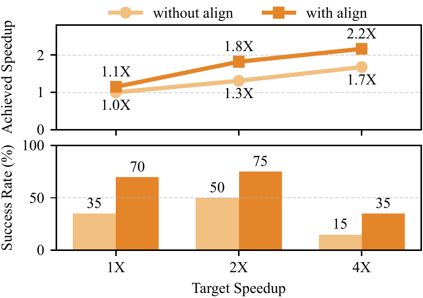
• Segment alignment is critical. Inference-time segment alignment keeps consecutive spline segments continuous, which is critical for stable high-speed execution. Without it, success becomes highly sensitive to speed as discontinuities push the policy out of distribution.

  

Simulation Benchmarks

We also evaluate BSP on Push-T, RoboMimic, and RoboCasa simulation tasks.

We find that BSP generally matches or improves baseline success rates across these simulation benchmarks.

Acknowledgements

We thank Minghuan Liu, Tiange Xiang for their helpful discussions.

Citation

To cite this work, please use the following BibTeX entry:

tbd